Photograph Scenario

The problem definition for the Spreadsheet for Large Images contained a number of scenarios setting out the purpose of the spreadsheet. One was about a photographic studio:

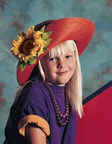
A photographic studio offers a digitisation and image manipulation service. One of the staff will be available to use the spreadsheet which must take a number of images and apply a range of different filters.

In this case the customer has brought in a range of recent snaps and wants some antique photographs created.

The photographs are scanned in so the spreadsheet can use them.

The first image can then be loaded into the spreadsheet by entering the formula, =LOAD("girl.jpg"), into cell A1 or by selecting the cell and using a menu short cut.

	A	B	C	D	E
1

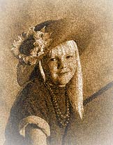
There are a couple of features that suggest a photograph in antique, black that has faded to brown and extra fading around the edges. Let us begin by producing a black and white image by entering =GRAYSCALE(A1) into cell B1.

	A	B	C	D	E
1

A brown image could be made by changing the colour balance of the black and white image but there is an easier way, combine the current image with a suitable panel of brown. Enter the formula =RGBIMAGE((68,101,13);DIMENSION(B1)) into C1 and =OVERLAY(B1;C1;85) into D1. The function RGBIMAGE produces an image using a separate red, green, and blue function on X and Y. In this instance all the functions are constant giving a brown panel with the same dimensions as B1. OVERLAY blends two images together, the brown image is given a percentage transparency and placed over the black and white girl.

	A	B	C	D	E
1

Fading at the edges can be made using a similar technique. Put formula =GAUSIANBLUR( APPLY( BWIMAGE(0;DIMENSION(D1)); BWIMAGE(1;SHRINK(DIMENSION(D1);(2,2))); 100);16) into E1 and =SCREEN(A4;A5;100) into F1. The first formula is rather complicated and comes in four parts. BWIMAGE(0;DIMENSION(D1)) creates a solid white image, BWIMAGE(1;SHRINK(DIMENSION(D1);(2,2))) creates a smaller solid black image, APPLY combines them to create a black image with a white border, and GAUSIANBLUR produces the final image using a large blur radius. The second formula combines the girl with the blur to produce a faded image.

	B	C	D	E	F
1

The final image looks reasonable but could be better if the picture had deteriorated over the years. We need to make a noisy grayscale image so we move the formulae in C1-F1 over to D1-G1. A short cut for this is to select the cells and use the hand cursor to drag them to their new location.

	B	C	D	E	F
1

An error icon appears to show where the formula in E1 no longer finds the image expected in C1. Noise can be added to the grayscale image by putting =NOISE(B1;20) into C1. The other images are recalculated using the noisy grayscale as a starting point.

	C	D	E	F	G
1

Now we have a suitable thumbnail image we can calculate the full-size version.

An image can be saved using another formula =SAVE(G1;"antique "&NAME(A1)). When the spreadsheet is closed this formula will save the full-size image with the name "antique girl". To create the other images all we need do is load the originals into cells B1-C1 and use the fill down menu option to replicate the formula. If we also switch the image of these cells off then the spreadsheet will not create the intermediate thumbnail images. Now, if the customer is happy with the images, they can be printed out from the saved files or directly by the spreadsheet.

Sometimes during this scenario particular parameters have been used for filters and the way to find such parameters is through experimentation. As the parameters are change the spreadsheet will recalculate all the affected thumbnail images so we can see the new effect. The properties of all of the functions within this example are assumed, none have yet been implemented within the spreadsheet.